Effective Python: R-Style Regression
I use R, but I love Python. However, let’s face it, basic linear regression in R is very straightforward. A few clear and intuitive lines of R code produce textbook1 output that is informative and complete. This post compares building and analyzing simple linear regression models in R and Python.
Sample data set
Let’s look at the data set Earnings.txt2 from the Data and Story Library. DASL is a great resource for test data. Earnings.txt includes the price, SAT, ACT, and graduate earnings for over 700 US colleges. .
Exploring the connection between the cost of college and future earnings is interesting in its own right and the post includes more models than needed for the R/Python comparison—I can’t resist—but the outputs are in the Appendix.
1. Ingestion and basic EDA
1.1. Ingestion and basic EDA in R
library(tidyverse)
# College cost vs earnings
df = read_tsv('C:/Users/steve/S/Teaching/2019-01/ACT3349/data/earnings.txt')
dfa = df %>% select(Price, Earn, SAT, ACT, Public)
head(dfa)

# A tibble: 6 x 5
#   Price  Earn   SAT   ACT Public
#   <dbl> <dbl> <dbl> <dbl>  <dbl>
# 1 61300 62800  1510    33      0
# 2 28100 59000  1380    30      1
# 3 64800 62900  1510    34      0
# 4 58600 63700  1460    33      0
# 5 35700 60300  1360    30      1
# 6 18500 51800  1260    29      1

summary(dfa)
#     Price            Earn            SAT            ACT            Public
# Min.   :16500   Min.   :28300   Min.   : 810   Min.   :15.00   Min.   :0.0000
# 1st Qu.:25900   1st Qu.:41100   1st Qu.:1040   1st Qu.:23.00   1st Qu.:0.0000
# Median :44000   Median :44750   Median :1120   Median :25.00   Median :0.0000
# Mean   :42200   Mean   :45598   Mean   :1142   Mean   :24.98   Mean   :0.3796
# 3rd Qu.:55500   3rd Qu.:48900   3rd Qu.:1220   3rd Qu.:27.00   3rd Qu.:1.0000
# Max.   :70400   Max.   :79700   Max.   :1550   Max.   :34.00   Max.   :1.0000
1.2. Ingestion and basic EDA in Python
import pandas as pd
# df = pd.read_csv('http://www.mynl.com/static/data/earnings.txt', sep='\t')
df = pd.read_csv('C:/Users/steve/S/Teaching/2019-01/ACT3349/data/earnings.txt', sep='\t')
dfa = df[['Price', 'Earn', 'SAT', 'ACT', 'Public']]
dfa.head()
#    Price   Earn   SAT  ACT  Public
# 0  61300  62800  1510   33       0
# 1  28100  59000  1380   30       1
# 2  64800  62900  1510   34       0
# 3  58600  63700  1460   33       0
# 4  35700  60300  1360   30       1

dfa.describe()
#          Price     Earn      SAT      ACT    Public
# count  706.000  706.000  706.000  706.000   706.000
# mean   42,200    45,598    1,142   24.982  0.379603
# std    15,727     6,724   136.572   3.451  0.485632
# min    16,500    28,300   810.000  15.000     0.000
# 25%    25,900    41,100    1,040   23.000     0.000
# 50%    44,000    44,750    1,120   25.000     0.000
# 75%    55,500    48,900    1,220   27.000     1.000
# max    70,400    79,700    1,550   34.000     1.000
1.3 Comparison
Neutral. I like getting standard deviation. Obviously, you’d do more EDA! Number formatting was not normalized.
2. Regression
2.1. Regression in R
m1 = lm(data=dfa, Earn ~ Price)
summary(m1)

# Call:
# lm(formula = Earn ~ Price, data = dfa)
#
# Residuals:
#      Min       1Q   Median       3Q      Max
# -16905.1  -4183.1   -921.5   3217.7  30777.6
#
# Coefficients:
#              Estimate Std. Error t value Pr(>|t|)
# (Intercept) 4.042e+04  6.951e+02  58.150  < 2e-16 ***
# Price       1.227e-01  1.544e-02   7.948 7.55e-15 ***
# ---
# Signif. codes:  0 ‘***’ 0.001 ‘**’ 0.01 ‘*’ 0.05 ‘.’ 0.1 ‘ ’ 1
#
# Residual standard error: 6446 on 704 degrees of freedom
# Multiple R-squared:  0.08234,   Adjusted R-squared:  0.08103
# F-statistic: 63.17 on 1 and 704 DF,  p-value: 7.552e-15
2.2. Regression in Python
m1 = smf.ols(formula='Earn ~ Price', data=df)
res1 = m1.fit()
res1.summary()

#                             OLS Regression Results
# ==============================================================================
# Dep. Variable:                   Earn   R-squared:                       0.082
# Model:                            OLS   Adj. R-squared:                  0.081
# Method:                 Least Squares   F-statistic:                     63.17
# Date:                Wed, 09 Feb 2022   Prob (F-statistic):           7.55e-15
# Time:                        10:39:37   Log-Likelihood:                -7193.2
# No. Observations:                 706   AIC:                         1.439e+04
# Df Residuals:                     704   BIC:                         1.440e+04
# Df Model:                           1
# Covariance Type:            nonrobust
# ==============================================================================
#                  coef    std err          t      P>|t|      [0.025      0.975]
# ------------------------------------------------------------------------------
# Intercept   4.042e+04    695.108     58.150      0.000    3.91e+04    4.18e+04
# Price          0.1227      0.015      7.948      0.000       0.092       0.153
# ==============================================================================
# Omnibus:                      114.947   Durbin-Watson:                   1.232
# Prob(Omnibus):                  0.000   Jarque-Bera (JB):              207.069
# Skew:                           0.977   Prob(JB):                     1.09e-45
# Kurtosis:                       4.794   Cond. No.                     1.29e+05
# ==============================================================================
2.3. Comparing R and Python regression code
- Call syntax: identical
- Extra
.fit()call could be included in the model,res1 = smf.ols(formula='Earn ~ Price', data=df).fit() - Output: comparable, though Python missing the residual standard error. It is available as
res1.scale ** 0.5(from GLMs where the scale acts like the variance).
My verdict: a tie.
3. Plotting
3.1. Plotting in R
require(gridExtra)
gp1 = ggplot(data=dfa, aes(x=Price, y=Earn, col=factor(Public))) + geom_point() + geom_smooth(method='lm')
gp2 = ggplot(data=dfa, aes(x=Price, y=Earn, col=SAT)) + geom_point() + geom_smooth(method='lm')
grid.arrange(gp1, gp2, ncol=2)
3.2. Plotting in Python
import matplotlib.pyplot as plt
fig, axs = plt.subplots(1, 2, figsize=(10, 3.5), tight_layout=True)
ax0, ax1 = axs.flat

ax = ax0
pred_ols3 = res3.get_prediction()
df['iv_l'] = pred_ols3.summary_frame(alpha=0.01)["mean_ci_lower"]
df['iv_u'] = pred_ols3.summary_frame(alpha=0.01)["mean_ci_upper"]
df['fit'] = res3.fittedvalues

x = df.Price
y = df.Earn
df.plot.scatter(x='Price', y='Earn', s=2, marker='o', c=df.Public, ax=ax, colorbar=False)
df.plot.scatter(x='Price', y='fit',  s=2, marker='o', c=df.Public, ax=ax, colorbar=False)
df.plot.scatter(x='Price', y='iv_l', s=2, marker='o', c=df.Public, ax=ax, colorbar=False)
df.plot.scatter(x='Price', y='iv_u', s=2, marker='o', c=df.Public, ax=ax, colorbar=False)
ax.legend()
ax.grid(lw=.25, c='w')

ax = ax1
pred_ols1 = res1.get_prediction()
iv_l = pred_ols1.summary_frame(alpha=0.01)["mean_ci_lower"]
iv_u = pred_ols1.summary_frame(alpha=0.01)["mean_ci_upper"]

df.plot.scatter(x='Price', y='Earn', s=2, marker='o', cmap='RdBu', c=df.SAT, ax=ax)
ax.scatter(x, res1.fittedvalues, s=1, c="r", marker='.', label="OLS fit")
ax.scatter(x, iv_u, s=2, c='b', marker='.', label="OLS 99% mean ci")
ax.scatter(x, iv_l, s=2, c='b', marker='.')

ax.grid(lw=.25, c='w')
ax = fig.axes[-1]
ax.set_title('SAT', fontsize=12)
ax.yaxis.set_major_locator(ticker.MultipleLocator(100))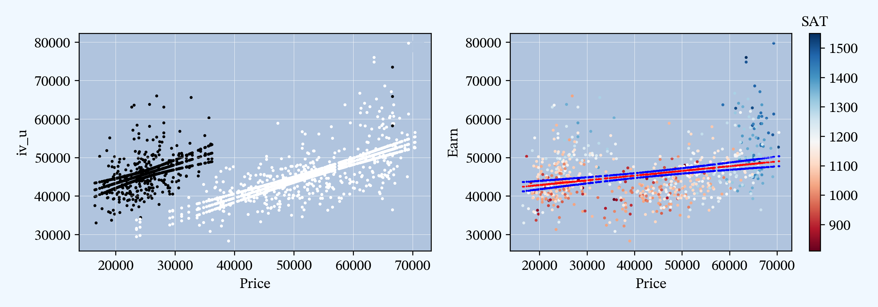
3.3. Comparison
Hummm, why do I love Python so much?
4. Conclusions
Appendix A. More data analysis
Is it worth paying more for a fancy college? Here are a few more model views to consider.
A.1. Further regressions in R
m2 = lm(data=dfa, Earn ~ Price + SAT)
summary(m2)

# Call:
# lm(formula = Earn ~ Price + SAT, data = dfa)
#
# Residuals:
#      Min       1Q   Median       3Q      Max
# -16325.5  -3546.6   -247.4   3202.0  24833.5
#
# Coefficients:
#              Estimate Std. Error t value Pr(>|t|)
# (Intercept) 1.461e+04  1.814e+03   8.055 3.41e-15 ***
# Price       6.177e-03  1.549e-02   0.399     0.69
# SAT         2.691e+01  1.783e+00  15.088  < 2e-16 ***
# ---
# Signif. codes:  0 ‘***’ 0.001 ‘**’ 0.01 ‘*’ 0.05 ‘.’ 0.1 ‘ ’ 1
#
# Residual standard error: 5606 on 703 degrees of freedom
# Multiple R-squared:  0.3068,    Adjusted R-squared:  0.3048
# F-statistic: 155.6 on 2 and 703 DF,  p-value: < 2.2e-16

m3 = lm(data=dfa, Earn ~ Price * factor(Public))
summary(m3)

# Call:
# lm(formula = Earn ~ Price * factor(Public), data = dfa)
#
# Residuals:
#    Min     1Q Median     3Q    Max
# -15745  -3827   -552   2699  26268
#
# Coefficients:
#                        Estimate Std. Error t value Pr(>|t|)
# (Intercept)           2.039e+04  1.467e+03  13.899  < 2e-16 ***
# Price                 4.768e-01  2.737e-02  17.422  < 2e-16 ***
# factor(Public)1       1.322e+04  2.317e+03   5.705 1.71e-08 ***
# Price:factor(Public)1 7.377e-03  7.561e-02   0.098    0.922
# ---
# Signif. codes:  0 ‘***’ 0.001 ‘**’ 0.01 ‘*’ 0.05 ‘.’ 0.1 ‘ ’ 1
#
# Residual standard error: 5502 on 702 degrees of freedom
# Multiple R-squared:  0.3333,    Adjusted R-squared:  0.3304
# F-statistic:   117 on 3 and 702 DF,  p-value: < 2.2e-16

m4 = lm(data=dfa, Earn ~ Price + factor(Public) + SAT)
summary(m4)

# Call:
# lm(formula = Earn ~ Price + factor(Public) + SAT, data = dfa)
#
# Residuals:
#    Min     1Q Median     3Q    Max
# -14885  -3365   -377   2924  23955
#
# Coefficients:
#                  Estimate Std. Error t value Pr(>|t|)
# (Intercept)     1.050e+04  1.743e+03   6.024 2.75e-09 ***
# Price           2.981e-01  3.217e-02   9.268  < 2e-16 ***
# factor(Public)1 9.355e+03  9.206e+02  10.162  < 2e-16 ***
# SAT             1.661e+01  1.950e+00   8.518  < 2e-16 ***
# ---
# Signif. codes:  0 ‘***’ 0.001 ‘**’ 0.01 ‘*’ 0.05 ‘.’ 0.1 ‘ ’ 1
#
# Residual standard error: 5238 on 702 degrees of freedom
# Multiple R-squared:  0.3957,    Adjusted R-squared:  0.3931
# F-statistic: 153.2 on 3 and 702 DF,  p-value: < 2.2e-16
A.2. Further regressions in Python
m2 = smf.ols(formula='Earn ~ Price + SAT', data=df)
res2 = m2.fit()
res2.summary()

#                             OLS Regression Results
# ==============================================================================
# Dep. Variable:                   Earn   R-squared:                       0.307
# Model:                            OLS   Adj. R-squared:                  0.305
# Method:                 Least Squares   F-statistic:                     155.6
# Date:                Wed, 09 Feb 2022   Prob (F-statistic):           1.14e-56
# Time:                        10:39:59   Log-Likelihood:                -7094.2
# No. Observations:                 706   AIC:                         1.419e+04
# Df Residuals:                     703   BIC:                         1.421e+04
# Df Model:                           2
# Covariance Type:            nonrobust
# ==============================================================================
#                  coef    std err          t      P>|t|      [0.025      0.975]
# ------------------------------------------------------------------------------
# Intercept   1.461e+04   1814.156      8.055      0.000    1.11e+04    1.82e+04
# Price          0.0062      0.015      0.399      0.690      -0.024       0.037
# SAT           26.9095      1.783     15.088      0.000      23.408      30.411
# ==============================================================================
# Omnibus:                       51.603   Durbin-Watson:                   1.662
# Prob(Omnibus):                  0.000   Jarque-Bera (JB):               80.196
# Skew:                           0.541   Prob(JB):                     3.85e-18
# Kurtosis:                       4.247   Cond. No.                     3.87e+05
# ==============================================================================

df["Pubic"] = df["Public"].astype("category")
m3 = smf.ols(formula='Earn ~ Price * Public', data=df)
res3 = m3.fit()
res3.summary()

#                             OLS Regression Results
# ==============================================================================
# Dep. Variable:                   Earn   R-squared:                       0.333
# Model:                            OLS   Adj. R-squared:                  0.330
# Method:                 Least Squares   F-statistic:                     117.0
# Date:                Wed, 09 Feb 2022   Prob (F-statistic):           1.97e-61
# Time:                        10:40:27   Log-Likelihood:                -7080.5
# No. Observations:                 706   AIC:                         1.417e+04
# Df Residuals:                     702   BIC:                         1.419e+04
# Df Model:                           3
# Covariance Type:            nonrobust
# ================================================================================
#                    coef    std err          t      P>|t|      [0.025      0.975]
# --------------------------------------------------------------------------------
# Intercept     2.039e+04   1466.843     13.899      0.000    1.75e+04    2.33e+04
# Price            0.4768      0.027     17.422      0.000       0.423       0.531
# Public        1.322e+04   2316.891      5.705      0.000    8669.333    1.78e+04
# Price:Public     0.0074      0.076      0.098      0.922      -0.141       0.156
# ==============================================================================
# Omnibus:                      123.249   Durbin-Watson:                   1.516
# Prob(Omnibus):                  0.000   Jarque-Bera (JB):              254.866
# Skew:                           0.979   Prob(JB):                     4.53e-56
# Kurtosis:                       5.198   Cond. No.                     5.57e+05
# ==============================================================================

m4 = smf.ols(formula='Earn ~ Price + Public + SAT', data=df)
res4 = m4.fit()
res4.summary()

#                             OLS Regression Results
# ==============================================================================
# Dep. Variable:                   Earn   R-squared:                       0.396
# Model:                            OLS   Adj. R-squared:                  0.393
# Method:                 Least Squares   F-statistic:                     153.2
# Date:                Wed, 09 Feb 2022   Prob (F-statistic):           2.19e-76
# Time:                        10:41:24   Log-Likelihood:                -7045.7
# No. Observations:                 706   AIC:                         1.410e+04
# Df Residuals:                     702   BIC:                         1.412e+04
# Df Model:                           3
# Covariance Type:            nonrobust
# ==============================================================================
#                  coef    std err          t      P>|t|      [0.025      0.975]
# ------------------------------------------------------------------------------
# Intercept    1.05e+04   1742.734      6.024      0.000    7075.906    1.39e+04
# Price          0.2981      0.032      9.268      0.000       0.235       0.361
# Public      9355.2181    920.576     10.162      0.000    7547.806    1.12e+04
# SAT           16.6125      1.950      8.518      0.000      12.783      20.441
# ==============================================================================
# Omnibus:                       80.685   Durbin-Watson:                   1.703
# Prob(Omnibus):                  0.000   Jarque-Bera (JB):              139.548
# Skew:                           0.734   Prob(JB):                     4.98e-31
# Kurtosis:                       4.610   Cond. No.                     4.02e+05
# ==============================================================================
Textbook is circular at this point; many textbooks use R output to illustrate!↩︎
Archived copy of the data.↩︎
posted 2022-02-09 | tags: R, regression, Python, Effective Python, matplotlib, statsmodels